Neshyba & de Miguel, 2023

An Introduction to Statistical Mechanics

A brief introduction to StatMech

Statistical Mechanics is the name coined by Josiah Willard Gibbs back in 1884 to describe a set of methods people were inventing at the time, which were aimed at using microscopic properties of substances to explain their macroscopic properties (see https://en.wikipedia.org/wiki/Statistical_mechanics). Nowadays, those microscopic properties tend to be atomic-level properties that we can observe from spectroscopy experiments (like IR absorption experiments), or that we can predict from calculations (e.g., by solving Schrödinger's Equation). The macroscopic properties that StatMech tries to explain cover a huge range of possibilities, including heat capacities, thermoconductivity -- any bulk property you can measure. A great triumph of StatMech has been to beat a path from microscopic properties that one might get from Quantum Mechanics, to all the state functions of Thermodynamics -- including the internal energy, $U$, the Gibbs energy, the entropy, and the enthalpy.

But first we'll need to develop some foundational tools, starting most fundamentally with how molecules store energy.

How molecules store energy

You probably remember that molecules vibrate with certain frequencies that you can get from an IR absorption experiment. An example is shown in Fig. 1.

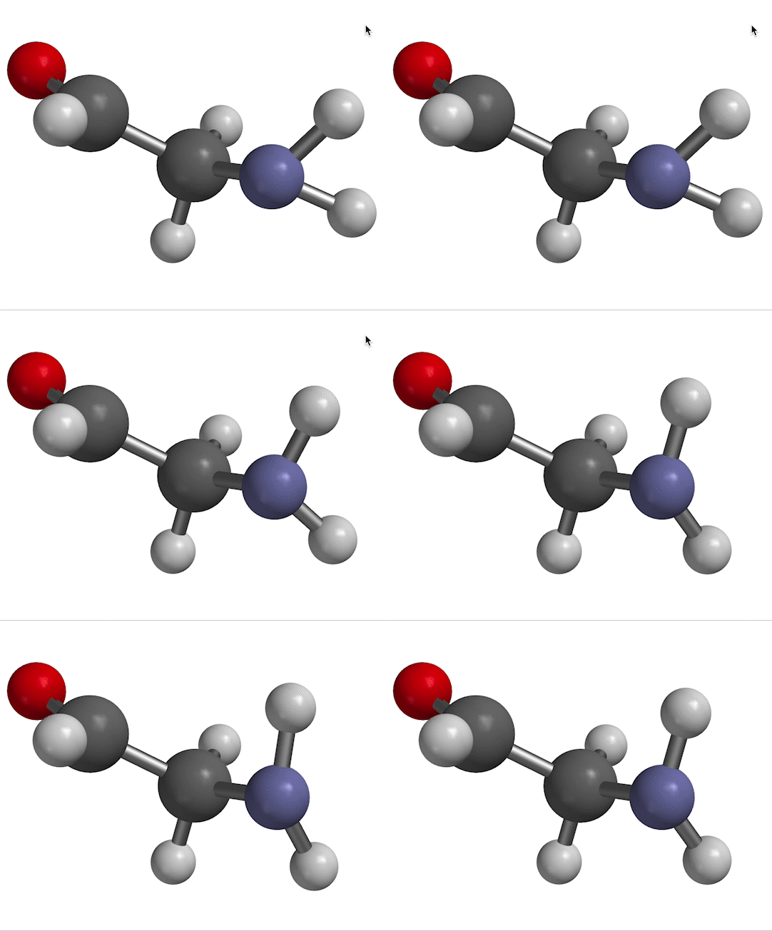Figure 1. NH$_2$ scissors motion of 2-aminoacetaldehyde, with water solvent represented as a homogeneous dielectric medium.

The motion we're looking at in Fig. 1 has a characteristic frequency of oscillation, which we typically designate with the symbol $\nu$. The same information appears in other forms, depending on the context. For example, in a typical IR spectrum, this motion would appear as a peak at wavenumber $\overline \nu$, given by

$$ \overline \nu = \nu/c \ \ \ \ (1) $$

Some people prefer to think in terms of angular frequencies,

$$ \omega = 2 \pi \nu \ \ \ \ (2) $$

These quantities tend to arise in quantum mechanics multipied by Planck's constant, where the math is just as simple one way or the other, since $h\nu=\hbar\omega$.

As for a quantum-mechanical analysis of this motion, a typical approximation (as you'll probably recall from previous work) is to describe the bending shown in Fig. 1 as a harmonic potential, ${1 \over 2}kx^2$ (where $x$ is the bending displacement you see in the figure). That information goes into Schrödinger's equation, which produces results like the ones shown in Fig. 2.

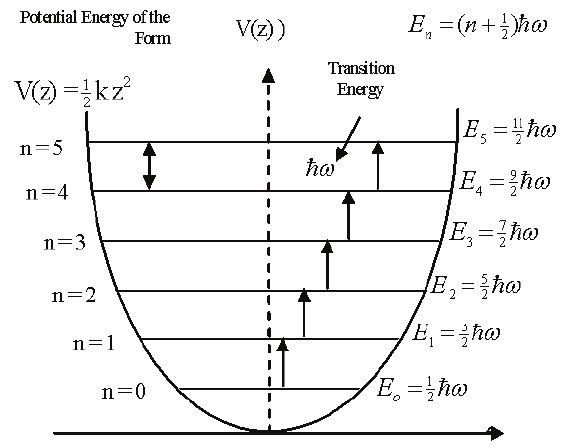Figure 2. Vibrational energy levels.

As Fig. 2 suggests, the eigenenergies associated with vibrational motion are given by

$$ E_n = (n + {1 \over 2}) h \nu = (n + {1 \over 2})\hbar \omega \ \ \ \ (3) $$

where $n=0,1,...$ As you can see, the energy gaps between states are all the same,

$$ E_{gap} = \hbar \omega N_A \ \ \ \ (4) $$

where we've tossed in Avogadro's number ($N_A$) to put these energies on a per-mole (rather than per-molecule) basis. So, if we wanted to focus on just the energy differences with respect to the ground state (which we do here), we could say

$$ \Delta E_n = n E_{gap} \ \ \ \ (5) $$

The Partition Function and state functions derived from them

The foundational quantity of StatMech is the partition function, to which we'll give the symbol $Z$ (it also appears in the literature as $Q$). What exactly is $Z$? In physical terms, you can think of it as the number of quantum states available to a system at a given temperature.

An intuitive (but rough) estimate of $Z$ can be got from comparing the energy gap relative to the ground state of a system that we were just talking about, to the energy available in a typical intermolecular collision. That second quantity is given by ${3 \over 2}RT$, which (at room temperature) is about 4 kJ/mol (but of course gets bigger or smaller as the temperature goes up or down). Now, referring to Fig. 3, we can predict the following

• At sufficiently low temperatures, ${3 \over 2}RT << \Delta E_n$, so intermolecular collisions would hardly ever have enough energy to bump molecules out of the ground vibrational state. In that case, we'd expect $Z\approx 1$.
• As temperature goes up, at some point we'd find that the energy of intermolecular collisions (remember that's ${3 \over 2}RT$) would get close enough to $\Delta E_n$ that collisions could bump molecules in the ground vibrational state up one. We could expect $Z$ to be about equal to two in that case (and so on).

Figure 3 shows the results of a more quantitative treatment, assuming a vibrating molecule that has $E_{gap} \approx 1$ kJ/mol.

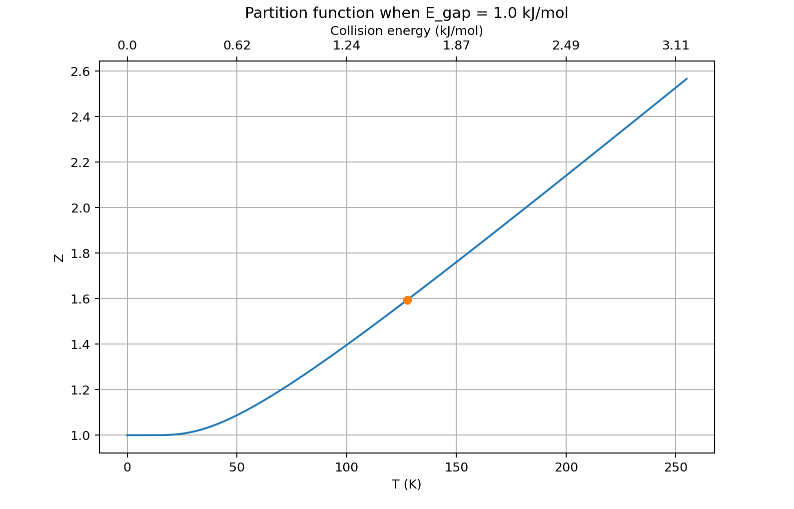Figure 3. Partition function $Z(T)$ of a vibrating molecule having an energy spacing between vibrational levels of ~1 kJ/mol.

You can see that when the temperature is high enough that the energy of a typical collision is a little more than the energy spacing between vibrational levels (the marker), between one and two quantum states are available ($Z\approx 1.6$). And of course that number keeps going up as the temperature rises.

How do we compute partition functions such as the one in Fig. 3? It's surprisingly simple, actually:

$$ Z = \sum_{n} e^{-\Delta E_n / RT} \ \ \ \ (6) $$

so as long as you know the energy levels $E_n$, you can find $Z$.

As advertised, the partition function can be used to derive expressions for all thermodynamic state functions. You can find a comprehensive list at https://en.wikipedia.org/wiki/Partition_function_(statistical_mechanics), but the one we'll need here is $U$,

$$ U = RT^2 {d \over dT} lnZ \ \ \ \ (7) $$

Application to thermophoresis

The context we'll be considering is called thermophoresis, a phenomenon first documented in the mid-1800s, but of considerable contemporary interest too. But what is thermophoresis? As described in https://en.wikipedia.org/wiki/Thermophoresis,

"The phenomenon is observed at the scale of one millimeter or less. An example that may be observed by the naked eye with good lighting is when the hot rod of an electric heater is surrounded by tobacco smoke: the smoke goes away from the immediate vicinity of the hot rod. As the small particles of air nearest the hot rod are heated, they create a fast flow away from the rod, down the temperature gradient. They have acquired higher kinetic energy with their higher temperature. When they collide with the large, slower-moving particles of the tobacco smoke they push the latter away from the rod."

Here we'll consider the thermophoresis of a solute dissolved in a solvent, sandwiched between two thermal reservoirs, such as depicted in Fig. 4.

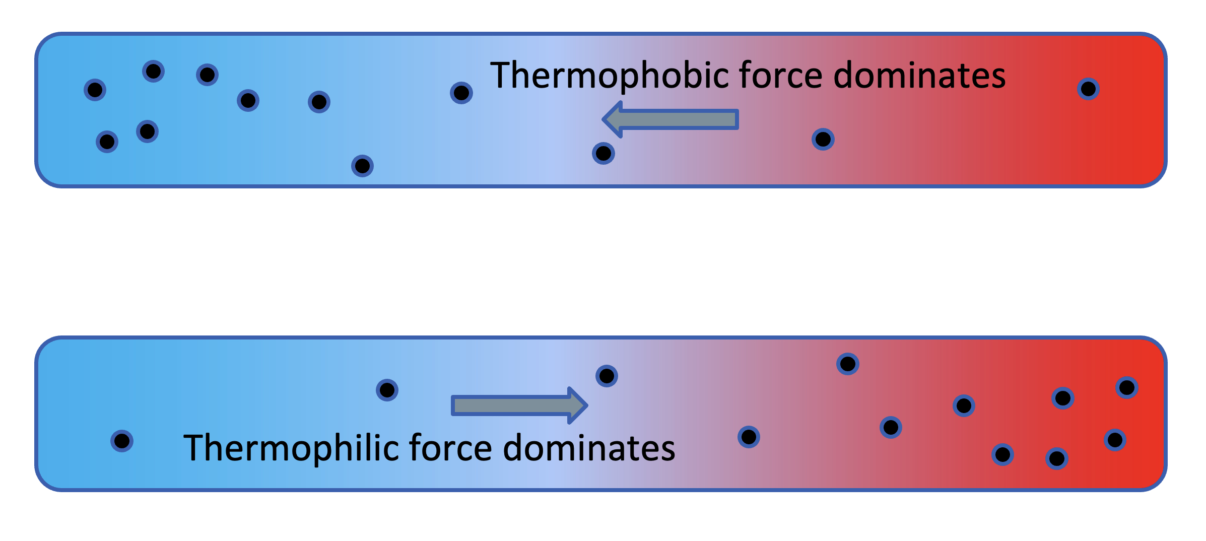Figure 4. Evidence of thermophoretic forces.

where the horizontal distance (call it $x$) spans a distance of (in this case) 0.1 cm. We're assuming an imposed, fixed temperature gradient as a function this distance,

$$ T(x) = T_{cold} + (T_{hot}-T_{cold}){x \over L} \ \ \ \ (8) $$

Two possibilities are indicated in the figure. Thermophobic thermophoresis is where the solute moves away from the heat. Thermophilic thermophoresis is where the solute moves toward the heat.

Which is the correct picture? StatMech's answer is to construct the energy of the solute, $U(T)$, where the temperature runs from hot to cold across some distance $L$ (Eq. 8). Then, analogously to the way a ball moves downhill in a gravitational field (Fig. 5), to predict that solute molecules will also move "downhill," toward lower values of $U(T)$.

Figure 5. Ball rolling downhill.

Temperature-independent vs temperature-dependent Hamiltonians

You can see from the foregoing that central to our analysis is the vibrational frequency (wavenumber) of our solute. How do we figure that out? Fortunately, Spartan can provide some answers, but there's a detail about this that we'll have to be cognizant of. It has to do with the temperature dependence of these vibrational motions.

$\overline \nu$ in the high-temperature limit. Because we think of high temperature as being a situation in which solvent water molecules form only short-lived hydrogen bonds to the solute, the solvent may as well be considered a homogeneous dielectric substance. Figure 1 was obtained in this way, in Spartan, by specifying "water" as a solvent. Therefore, we'll call the wavenumber we get for the scissor bend in this manner $\overline \nu_{HT}$.

If we are happy with this picture, the thermophoretic analysis is pretty straightforward. We form the partition function according to Eq. 6, using a constant $\overline \nu_{HT}$, and inspect the resulting $U(x)$ -- if we see that it slopes down to the left (the cold side), we can conclude that the solute is thermophobic. If we see that $U(x)$ slopes down to the right, it's thermophilic!

$\overline \nu$ in the low-temperature limit. On the other hand, if you inspect Fig. 6, you'll see that there's another way to find the frequency of vibration. When you set things up with solvent molecules explicitly this way, the result is considered a low-temperature limit. That's because now, the solvent water molecules can form long-lived hydrogen bonds to the solute. We'll call the wavenumber we get for the scissor bend in this case $\overline \nu_{LT}$.

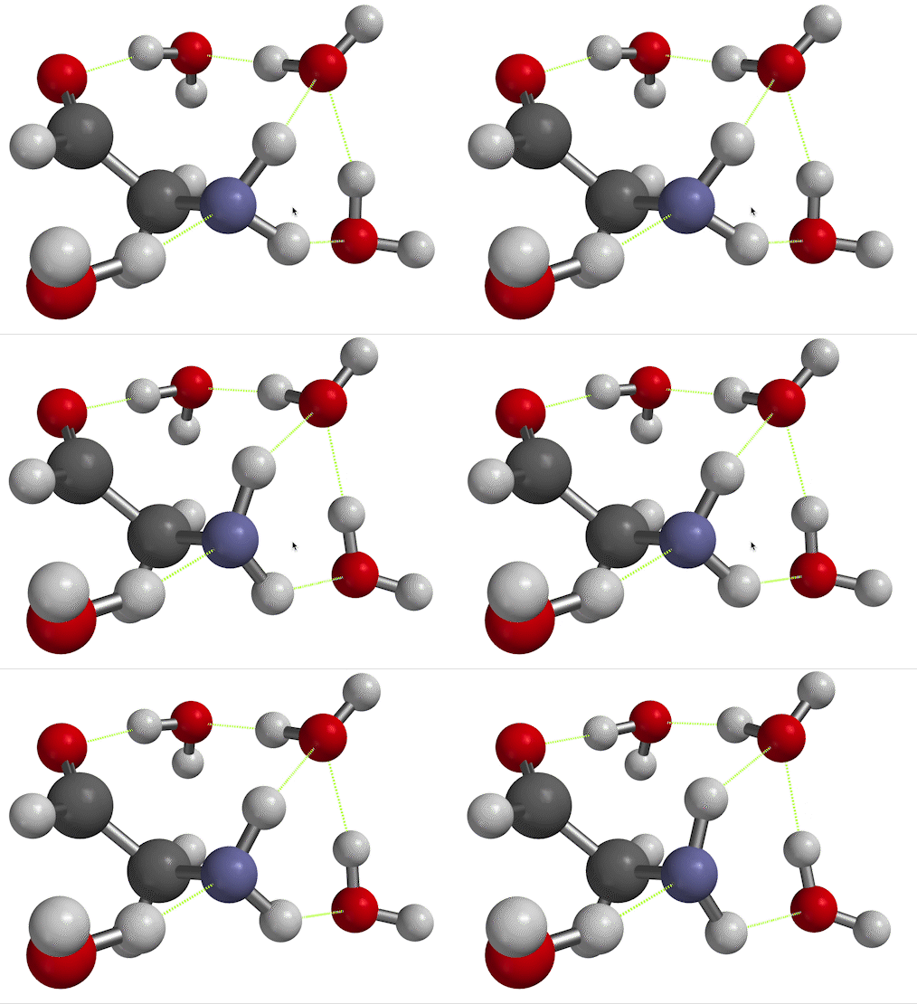Figure 6. NH$_2$ scissors motion of 2-aminoacetaldehyde, in which the water solvent has been represented explicitly as well as implicitly.

We'll also need a way to represent the transition from low temperature to high temperature. One possibility -- a sigmoidal transition -- is shown in Fig. 7.

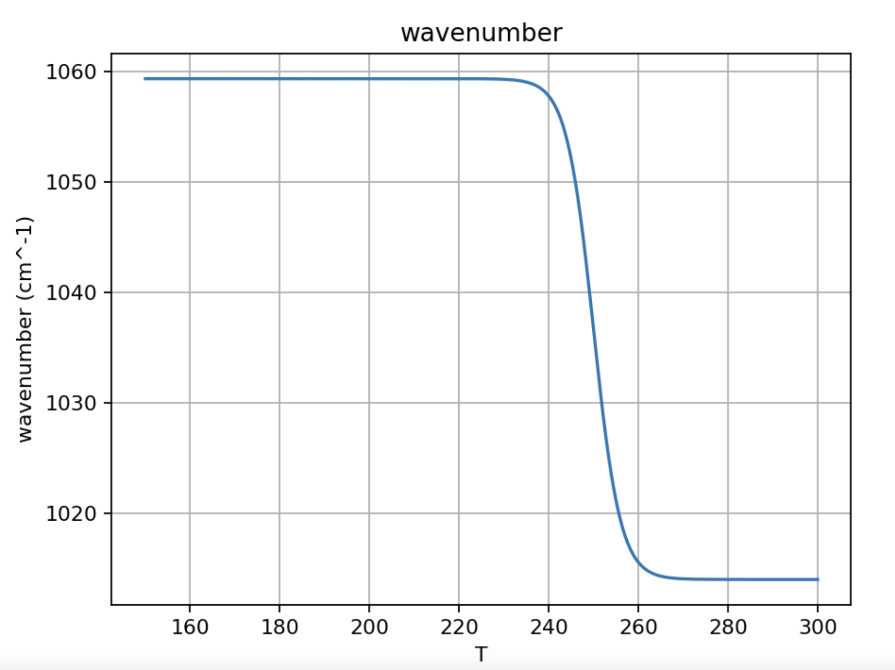Figure 7. Sigmoidal temperature dependence of the vibrational frequency of an aqueous solute. The left-hand, low-temperature limit is designated $\overline \nu_{LT}$, the right-hand, high-temperature limit is designated $\overline \nu_{HT}$.

The thermophoretic analysis in this case here is almost the same as before, with the exception that because the frequencies of vibration are temperature-dependent, Eq. 6 becomes $Z = \sum_{n} e^{-\Delta E_n(T) / RT}$, where we've written $E_n=E_n(T)$ to emphasize this difference.

Idea of this CGI

The main idea of this CGI is to use Statistical Mechanics to predict the thermophoretic properties of a solute. There will be Spartan and Python components:

• In Spartan, you'll construct a solute molecule containing an amine group, and find the frequency of its scissors vibration assuming water as a solvent (first implicitly only, then surrounded by water molecules as an explicit solvent).
• In Python, you'll figure out whether the thermophoretic forces acting on a that solute are thermophyllic or thermophobic, first assuming temperature-independent vibrations (i.e., the high-temperature limit), and then assuming temperature-dependent vibrations (i.e., transitioning from the low-temperature limit to the high-temperature limit by means of a sigmoidal function).

Learning goals

The main learning goals of this exercise are

1. I can construct state spaces needed for a StatMech problem.
2. I can explain what the thermophoretic force is, including its thermophyilic an thermophobic versions.
3. I can compute the energies, partition functions, and internal energy.
4. I can interpret $U(T)$ in terms of thermophoretic forces.

import pint; from pint import UnitRegistry; AssignQuantity = UnitRegistry().Quantity
import numpy as np
import plotly.graph_objects as go
import PchemLibrary as PL
import matplotlib.pyplot as plt
%matplotlib notebook

# Constants
R = AssignQuantity(8.314e-3,'kjoule/mol/K')
NA = AssignQuantity(6.02e23,'1/mol')
kB = R/NA
c = AssignQuantity(3.0e8,'m/s')
hbar = AssignQuantity(1,'atomic_unit_of_time * hartree'); print(hbar)
h = hbar*2*np.pi; print(h)

# The temperature range
T_cold = AssignQuantity(230,'K')
T_hot = AssignQuantity(310,'K')

Part 1. State space

Below is a tool that will come in handy for computing gridded variables (in this case, xgrid and ygrid) that span the ranges indicated. Study the results a bit to get a feel for how it works.

# An example of how it works
xgrid,ygrid = PL.Statespace([0,3,4],[0,2,3])
xgrid = AssignQuantity(xgrid,'meter')
ygrid = AssignQuantity(ygrid,'meter')
print('xgrid =\n', xgrid)
print('ygrid =\n', ygrid)

Your turn

Use Statespace to create a couple of gridded variables, in which the rows (x) run from 0 to 1 meters, with 11 steps, and the columns (y) run from 0 to 5 meters, with 6 steps. Call your variables xgrid and ygrid, since we'll using these a bit more in the cells below.

# Your code here 

Summing over state-space variables

The cell below shows how to sum the ygrid statespace variable over rows. To sum over columns, set the axis to 1.

# Summing over rows
sum_ygrid_over_rows = np.sum(ygrid,axis=0); print(sum_ygrid_over_rows)

# Summing over columns
# Your code here 

Pause for analysis

Why are there six values in the first array, but eleven in the second?

YOUR ANSWER HERE

Visualizing functions in state space

The cell below shows how to visualize $x^2(x,y)$.

# Visualizing the quantum numbers n on this state space
zgrid = xgrid**2
PL.plot3d(xgrid,ygrid,zgrid,xaxis_title='x',yaxis_title='y',zaxis_title='x^2')

Your turn

In the cell below, visualize $y^3(x,y)$, and update the z-label appropriately.

# Your code here 

Your turn

In the cell below, visualize $xy^2(x,y)$, and update the z-label appropriately.

# Your code here 

Pause for analysis: the idea of separability

The first two of these functions exhibit separability, while the third does not. Describe how you would know if a function $f(x,y)$ were separable, based on its graphical representation alone.

YOUR ANSWER HERE

Specifying our system's state space

In the cell below, create a state space in which the rows consists of 25 dimensionless vibrational quantum number values ($n$) spanning 0 to 24, and the columns consist of 101 distances ($x$) spanning 0 to 0.1 cm.

For simplicity, let's call these variables just "n" and "x" (even though they're both gridded variables).

# Your code here 


# This will be handy for later use
L = np.max(x); print(L)
dx = x[0,1]-x[0,0]; print(dx)

Visualizing our state space

In the cells below, visualize the state-space functions indicated, with appropriate labeling. Note -- you might have to rotate the graph to see anything.

# Visualize n(n,x)
# Your code here 


# Visualize x(n,x)
# Your code here 


# Construct T(n,x) and visualize it
# Your code here 


# This will be handy later
Tarray = T[0,:]; print(Tarray)
dT = Tarray[1]-Tarray[0]; print(dT)

Part 2. Thermophoresis assuming constant vibrational frequencies

You'll start this part in Spartan. Your goal is to carry out high-temperature study of the vibrational motion of a solute of your choice (but something with an amine group is recommended).

The first cell below shows how to construct a state-space function assuming this high-temperature limit of the frequency applies to all temperatures (we'll fix this later). You should modify it with the actual wavenumber you get from Spartan. This graph you get will be a bit boring since this is just a constant wavenumber, but later, when we invoke temperature-dependent frequencies, it'll get more interesting!

# This makes a gridded version of the wavenumber of vibration of your solute
# nubar_HT = AssignQuantity(1589,'1/cm')
nubar_HT = AssignQuantity(3618,'1/cm') # OH stretch of methanol

nubar = np.ones(np.shape(x))*nubar_HT
PL.plot3d(n,x,nubar,xaxis_title='n',yaxis_title='x',zaxis_title='nubar (High T)')

Energy of our oscillator

Below, your task is to construct and visualize the energy of your oscillator, $E_n(n,x)$, assuming a constant, high-temperature wavenumber for its vibration. You should convert it to kJ/mol.

# Compute En in the high-temperature limit (call it En_HT)
# Your code here 

Now the partition function

To do this, you'll need to construct the exponential quantity appearing in Eq. 6, and then carry out the summation (over axis 0) to get $Z(n,x)$. The Zarray you get from this should be just a function of temperature, since you're summing over quantum numbers $n$.

# Finding the partition function -- call it Zarray
# Your code here 


# Visualizing Zarray
plt.figure()
# plt.semilogy(Tarray,Zarray)
plt.plot(Tarray,Zarray)
plt.grid(True)
plt.xlabel('T')
plt.ylabel('Z')
plt.title('Partition function')

Pause for analysis

You'll probably notice that $Z(n,x)$ hardly budges from 1. Why is that?

YOUR ANSWER HERE

$U(T)$ from the partition function

The cell below has you calculate $U(T)$ from the partition function.

# Calculate U(T) from the partition function (call it Uarray)
# Your code here 


# Here we're plotting it on a semilog scale
plt.figure()
plt.semilogy(Tarray,Uarray,label='U(T)')
plt.grid(True)
plt.xlabel('T ('+str(Tarray.units)+')')
plt.ylabel('U ('+str(Uarray.units)+')')
plt.legend()

Pause for analysis

Is your solute thermophylic or thermophobic? How do you come to that conclusion?

YOUR ANSWER HERE

Part 3. Thermophoresis assuming temperature-dependent frequencies

A handy function

To represent the sigoidal function shown in Fig. 7, we've written a Python function shown below. Mathematically, it does this:

$$ f_{sigmoid}(T) = f_2 - (f_2-f_1) \times \bigl (1 - {1 \over 1 + e^\alpha} \bigr ) $$

where $\alpha = {T - T_{trans} \over T_{interval}}$, and $f$ is the wavenumber, $\bar \nu$, of the vibrational motion.

def f_sigmoid(f1, f2, T, T_transition, T_interval):
    sigmoid_arg = (T-T_transition)/T_interval    
    f = f2 - (f2-f1)*(1 - 1.0/(1.0 + np.exp(-sigmoid_arg)))
    return f

Using f_sigmoid

The cell below shows how to use our sigmoid function.

xarray = np.linspace(0,5)
y_of_x = f_sigmoid(2,1,xarray,2.5,0.2)
plt.figure()
plt.plot(xarray,y_of_x)
plt.grid(True)

Pause for analysis

You should play with the cell above to get a feel for what all the parameters in the sigmoid function do.

Constructing a temperature-dependent wavenumber function

In the cell below, construct a temperature-dependent function of frequencies, ranging from your low-temperature limit to your high-temperature limit, transitioning at a temperature of (say) 277 K, with a transition temperature interval of (say) 5 K.

The temperature variable to use in your call to f_sigmoid is the gridded temperature variable, $T$.

# Specify your low-temperature limit (but modify this to match your Spartan result)
# nubar_LT = AssignQuantity(1630,'1/cm')
nubar_LT = AssignQuantity(3177,'1/cm')

# Calculate a temperature-dependent wavenumber of vibration for the solute (call it nubar)
# Your code here 


# Plot it
PL.plot3d(n,x,nubar,xaxis_title='n',yaxis_title='x',zaxis_title='nubar (High T)')

Pause for analysis

Hopefully, you're looking at a wavenumber that transitions from one value to another as a function $x$, but is independent of $n$. Is it?

YOUR ANSWER HERE

Energies from angular frequencies

Below, calculate and visualize in 3d the energies of the oscillator, $E_n(n,x)$, based on the grid of angular frequencies you jsut created. You should get a result that looks a lot like the $E_n(n,x)$ you got before, but with a little bit of non-separability.

# Your code here 

Now the partition function

The Zarray you get from this should be (as previously) just a function of temperature, since you're summing over quantum numbers $n$.

# Calculate the partition function
# Your code here 


# Visualize the partition function
# Your code here 

U(T) from the partition function

Below, calculate $U(T)$ and plot it on a semilog scale (just like we did before).

# Your code here 

Pause for analysis

• Is your solute thermophylic or thermophobic, or a little of both?
• If you think about these results, you may be able to tell that solute will tend to accumulate at a particular location along the x-axis. What location is that?

YOUR ANSWER HERE

Refreshing and saving your code

1. Use the dropdown menu Kernel/Restart
2. Use the dropdown menu Cell/Run All Above
3. Under the "File" dropdown menu item in the upper left is a disk icon. Press it now to save your work (you can, do this at any time as you're working on an assignment, actually).

Validating

This step will help ensure that you didn't miss something (although it's not a guarantee). Find the "Validate" button and press it. If there are any errors or warnings, fix them.

Finishing up

Assuming all this has gone smoothly, carry out three more steps (but read this carefully before starting):

1. Close this notebook using the "File/Close and Halt" dropdown menu
2. Using the Assignments tab, submit this notebook
3. Press the Logout tab of the Home Page